Statistics in Engineering: Hypothesis Testing (Part 3 of 8)

Preface
This series is aimed at providing tools for an electrical engineer to gain confidence in the performance and reliability of their design. The focus is on applying statistical analysis to empirical results (i.e. measurements, data sets).

Introduction
This article will show step by step how to use hypothesis testing by using a before and after measurement to test the validity of a design change. For example you've change the amount of capacitance on your power supply rail and you've measured a lower average ripple voltage. Is this due to random variation or because you changed your design?

I don't think hypothesis testing is always necessary. If you change a resistor value in a voltage divider and the output changes by an order of magnitude you can be confident the change was the result of the value change. But it can be useful when your measurement hasn't changed much or the circuit is highly variable. The essence of what we are testing for is did the "after" measurement change enough to be considered significant?

Note: While these examples are Gaussian, Binomial distributions can be analyzed in the exact same way.

If you are not familiar with statistics or need a brush up I recommend Schaum's Statistics. It provides a good overview of material without a lot of time spent on proofs and lots of examples.

Concepts
Null Hypothesis, H₀: This whole approach begins with two data sets. One is a measurement of the original design and the second is a measurement post design change. We then start with an assumption that the shift in the measurement was due to random variation and not the design change. Again, we will begin by assuming that the design change had no effect. This assumption is called the null hypothesis. Once we formulate our null hypothesis we test it.

Level of Significance: The level of significance is the degree to which we are confident that our analysis is correct. For example a level of significance of 0.01 (99%) would indicate we are 99% certain the analysis is correct. There is no 100% certainty with a hypothesis test so choose a level appropriate to your situation. In other words did the new measurement differ by an appropriate number of sigmas?

One-tailed, Two-tailed: This is statistics speak for a test that is either >=x or <=x (one-tailed) or +/-x (two-tailed).

p-value: The probability of getting a value more extreme than your test (the "after" measurement).

Importing Your Data Set
I will use the R software package for statistical analysis. It is cross platform, free and open source. There are several Excel plugins which are good and if you have/can use SAS by all means use it.

The first row of your data set should be the titles for each column. Each column can contain anything but for building a distribution we can assume a single column with a row for each measurement.

NOTE: The following assumes the first column is the original data 'original' and the second column is the design change 'change'.


> rail_ripple<-read.csv(file.choose())
> dim(rail_ripple)
[1] 1000 2
> tail(rail_ripple)
original change
995 0.099504391 0.036869920
996 0.075531355 0.152026868
997 0.087253742 0.031136151
998 0.076154863 0.086135494
999 0.004237002 0.033424119
1000 0.095323337 0.001529153
> str(rail_ripple)
'data.frame': 1000 obs. of 2 variables:
$ original: num 0.0299 0.1212 0.0122 0.0652 0.0328 ...
$ change : num 0.0527 0.0572 0.0248 0.018 0.0524 ...
> attach(rail_ripple)


Calculate Mean and Sigma
Calculate your mean and sigma values.

For the original circuit:

> mean(original)
[1] 0.05761133
> sd(original)
[1] 0.03939702


For the new circuit:

> mean(change)
[1] 0.04769776
> sd(change)
[1] 0.03215615


We can see right away that the mean voltage ripple in the new circuit is lower by a bit. While it might be tempting to conclude it is in fact lower we will use statistics to determine how confident we are of that conclusion.

Calculate Sampling Distribution for Original Measurement
To illustrate this let's think about what we've actually done: calculated two results by averaging many values. And we know that if we take more measurements we will get a different mean and sigma every time. Because we are working with mean values what we really want to know is the distribution of the mean voltage ripple. This can be accomplished by taking many, many measurements of the original design -OR- it can be deduced from our original data set. If we have a distribution of means of the original design and the mean value of our design change we can visually see how likely our "after" measurement was due to the design change or chance.

The calculation is based on a distribution of mean values. Our distribution mean and sigma are calculated below:


> mean(original)
[1] 0.05761133
> mean(original)/sqrt(1000)
[1] 0.00182183


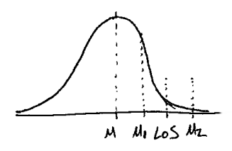
If the "after" result is mu₁ the variation may be due to random chance.
If the "after" result is mu₂ the variation may be due to design change.

Test Definition
Now that we have some footwork out of the way we setup our hypothesis test:

H₀: The design change had no effect on ripple.
- mean = 0.05761133 [V]
H₁: The design change lowered ripple.
- mean < 0.05761133 [V]

Because H₁ is "less than" this is a one-tailed test. Our sample size is 1000 and we are going for a level of significance of 0.001 (99.9%).

z Calculations
Formula: z = (mu - sample-mu)/mean_sigma

Design Change

> (mean(change)-mean(original))/(sd(original)/sqrt(1000))
[1] -7.957315


Level of Significance
A one-sided level of significance of 99.9% is:

> -qnorm(1-.001)
[1] -3.090232


Hypothesis Test and p-value
We can see that the new data is almost 8 sigmas from the mean and that our 99.9% null hypothesis was only ~3 sigmas away. It is quite unlikely that this is caused by random data. Therefore we are going to reject the null hypothesis that the design change had no effect.

This and many more examples of hypothesis testing are excellently documented at the R-Tutor website.

Small Sample Sizes
We can see from the example above that a large sample size helps us because large sample sizes build very tight (or tall and narrow) distributions of means. This allows us to more confidently establish whether or not a design change was responsible for a change in average values.

A sample size of only 100 would have resulted in the following result:

> (mean(change)-mean(original))/(sd(original)/sqrt(100))
[1] -2.516324


which gives us much less certainty about your design change.

When working with small sample sizes (<30) you can substitute the t statistics for the z statistics. t statistics are similar to normal distributions but tend to have "fatter" tails. The actual distribution of a t distribution is a function of the sample size so it takes into account the error introduced by a small sample size. A t distribution approaches a normal distribution as the sample size increases.

The process for hypothesis testing is identical except you use the following t formula (where N is the sample size) instead of the z formula:

> (mean(change)-mean(original))/(sqrt(N/(N-1))*sd(original))
[1] -2.516324


The confidence interval for sigma for small sample sizes is calculated as follows: > mean(original)+t*sd(original)/sqrt(N-1). To calculate t distributions use the qt and t.test functions.

And the confidence interval for sigma is available using the chi-squared function:

> sqrt(0.006329213^2*98973/qchisq(.995,df=(98973-1)))
[1] 0.006292799
> sqrt(0.006329213^2*98973/qchisq(.005,df=(98973-1)))
[1] 0.006366088


Next Up
So far we've either described a data set or compared two separate data sets. But how do we establish a relation between table data where we aren't sampling but instead we are counting? The answer lies with contingency testing and the chi-square distribution.